WBlog

wangzhiwei blog

0%

tfjs-study

机器学习是什么?

1
2
3
4
5
6
7
8
机器学习是对能通过经验自动改进的计算机算法的研究。

机器学习是研究
机器学习是计算机算法的研究
机器学习是对(经验)自动改进的计算机算法的研究。

机器学习是用(数据)或以往的(经验),以此优化计算机程序的性能标准。

机器学习例子 - 线性回归

1

机器学习例子 - 逻辑回归

机器学习例子 - 图片分类

机器学习例子 - 语音助手

为何要用机器学习?

有些棘手问题只能用机器学习来解决
获取数据比编写规则更容易
GPU等计算能力显著提升

机器学习如何运作?

神经网络 (重点)

2、决策树、支持向量机、贝叶斯分类器、强化学习…

神经网络

什么是神经网络?

在本课程中,指的是人工神经网络

人工神经网络是一种运算模型(就是输入输出的映射),由大量的节点(或称神经元)之间相互连接构成

在上图中显示的是双层神经网络

每个神经元里存储着若干 权重(weight)、偏置(bias)和一个激活函数(activation function)

计算过程:输入乘上权重,加上偏置,再经过激活函数得到输出

激活函数 用于添加一些非线性变化,不能一直线性增长

神经网络通常包括一个输入层、若干个隐藏层、一个输出层

输入层通常不用于计算神经网络的层数

什么是神经网络训练?

给大量输入和输出,算出神经网络里所有神经元的权重和偏置,然后给定新的输入,可以算出新的输出
在机器学习里输入输出被称为特征和标签,大量的输入和输出被称为训练集

例子:
给1000个相亲对象的数据(特征),和对应的满意程度(标签),训练完后,给一份新的相亲对象的数据,就可以判定满意程度了。

如何训练神经网络?

初始化:随机生成一些权重和偏置
计算损失:给定特征,计算出标签,得到它与真实标签的差距
优化:微调权重和偏置,让差距(损失)变小

前向传播与反向传播
前向传播:将训练数据的特征输入到神经网络,得到预测的标签
反向传播:将预测的标签与真实标签比较,得到损失,然后根据损失微调权重和偏置,让差距变小 (计算损失并优化)

如何计算损失?

使用损失函数
本课称涉及的损失函数:均方误差、对数损失、交叉熵损失
了解原理即可,工作中可以直接从第三方库中调用。tensorflow.js 中调用

如何优化?

使用优化器
本课称涉及的优化器:随机梯度下降(SGD)、Adam
了解原理即可,工作中可以直接从第三方库中调用。tensorflow.js 中调用

tensorflow.js 是什么

tensorflow.js 是一个开源的机器学习库,基于 TensorFlow 的 JavaScript 实现。
可以直接在浏览器和Node.js 中使用机器学习技术了

tensorflow.js 具体功能

运行现有模型
重新训练现有模型
使用 JavaScript 开发机器学习模型

什么是 Tensor ?

中文名叫张量
张量是向量和矩阵向更高维度的推广
相当于多维数组

1
2
3
4
5
6
7
import * as tf from '@tensorflow/tfjs';


const t0 = tf.tensor(1);
t0.print();
console.log(t0);

1
2
3
4
5
const t1 = tf.tensor([1, 2]);
t1.print();

console.log(t1);

1
2
3
4
5
6
7

const t2 = tf.tensor([[1, 2], [3, 4]]);

t2.print();
console.log(t2);


Tensor和机器学习的关系

神经网络的每一层要存储N维数据
N层的For循环运算
Tensor作为高维数据结构完美解决以上问题

1
2
3
4
5
6
7
8
9
10
11
12
13
14
15
16
17
18
19


import * as tf from '@tensorflow/tfjs';

// 传统 for 循环
const input = [1, 2, 3, 4];
const w = [[1, 2, 3, 4], [2, 3, 4, 5], [3, 4, 5, 6], [4, 5, 6, 7]];
const output = [0, 0, 0, 0];

for (let i = 0; i < w.length; i++) {
for (let j = 0; j < input.length; j++) {
output[i] += input[j] * w[i][j];
}
}

console.log(output);

tf.tensor(w).dot(tf.tensor(input)).print();

什么是线性回归?
利用数理统计中回归分析,来确定两种或两种以上变量间相互依赖的定量关系的一种统计分析方法。

例子:身高体重预测、房价预测

操作步骤
准备、可视化训练数据

使用TensorFlow.js的API 构建神经网络(只有一个神经元)

训练模型并预测

tf-vis 文档
https://js.tensorflow.org/api_vis/1.5.1/#render.scatterplot

定义模型结构:

单层单个神经元组成的神经网络

linear-study
.
├── dist
├── index.html
├── node_modules
├── package-lock.json
├── package.json
└── script.js

1
2
3
4
5
6
7
8
9
10
11
12
13
14
index.html

<!DOCTYPE html>
<html lang="en">
<head>
<meta charset="UTF-8">
<meta name="viewport" content="width=device-width, initial-scale=1.0">
<title>Document</title>
</head>
<body>
<script src="script.js"></script>
</body>
</html>

1
2
3
4
5
6
7
8
9
10
11
12
13
14
15
16
17
18
19
20
21
22
23
24
25
26
27
28
29
30
31
32
33
34
35
36
37
38
39
40
41
import * as tfvis from '@tensorflow/tfjs-vis';

window.onload = function () {

const xs = [1,2,3,4]
const ys = [1,3,5,7]

tfvis.render.scatterplot(
{ name: 'Linear Regression' },
{ values: xs.map((x, i) => ({ x, y: ys[i] })) },
// {
// xLabel: 'X',
// yLabel: 'Y',
// height: 300,
// },
{
xAxisDomain: [0, 10],
yAxisDomain: [0, 10]
}
);


// const model = tf.sequential(); //创建模型 (连续的模型)
// model.add(tf.layers.dense({ units: 1, inputShape: [1] })); //添加层 dense全连接层 输入维度为1 输出维度为1 units为输出维度 units 神经元的个数 https://js.tensorflow.org/api/4.22.0/#layers.dense
// model.compile({ loss: tf.losses.meanSquaredError, optimizer: tf.train.sgd(0.1) }); //编译模型 meanSquaredError MSE 均方误差损失函数 sgd 随机梯度下降 优化器
//
// const xs = tf.tensor2d([0, 1, 2, 3], [4, 1]);
// const ys = tf.tensor2d([0, 1, 2, 3], [4, 1]);

// const container = {
// name: 'Linear Regression',
// styles: {
// height: '1000px',
// width: '1000px',
// },
// };

// const surface = tfvis.visor().surface(container);


}

cnpm i parcel-bundler -g

parcel index2.html

cnpm 安装 @tensorflow/tfjs 报错,改为

npm install @tensorflow/tfjs 就没问题了

线性回归,训练模型并可视化训练过程

1
2
3
4
5
6
7
8
9
10
11
12
13
14
15
16
17
18
19
20
21
22
23
24
25
26
27
28
29
30
31
32
33
34
35
36


import * as tf from '@tensorflow/tfjs';
import * as tfvis from '@tensorflow/tfjs-vis';

window.onload = async () => {
const xs = [1, 2, 3, 4];
const ys = [1, 3, 5, 7];

tfvis.render.scatterplot(
{ name: '线性回归训练集' },
{ values: xs.map((x, i) => ({ x, y: ys[i] })) },
{ xAxisDomain: [0, 5], yAxisDomain: [0, 8] }
);

const model = tf.sequential();
model.add(tf.layers.dense({ units: 1, inputShape: [1] }));
// sgd 是随机梯度下降 meanSquaredError 是均方误差
model.compile({ loss: tf.losses.meanSquaredError, optimizer: tf.train.sgd(0.1) });

const inputs = tf.tensor(xs);
const labels = tf.tensor(ys);
await model.fit(inputs, labels, {
batchSize: 4,
epochs: 200,
callbacks: tfvis.show.fitCallbacks(
{ name: '训练过程' },
['loss']
)
});

const output = model.predict(tf.tensor([5]));
alert(`如果 x 为 5,那么预测 y 为 ${output.dataSync()[0]}`);
};

什么是归一化

把大数量级特征转化到较小的数量级下,通常是 0-1 之间,或者 -1-1 之间。

绝大多数 TensorFlow.js 模型都不是给特别大的数设计的

将不同数量级的特征归一化到同一数量级,防止某个特征影响过大

例子:身高体重预测、房价预测

准备身高体重训练数据并归一化

训练模型并预测,将结果反归一化为正常数据

1
2
3
4
5
6
7
8
9
10
11
12
13
14
15
16
17
18
19
20
21
22
23
24
25
26
27
28
29
30
31
32
33
34
35
36
37

import * as tf from '@tensorflow/tfjs';
import * as tfvis from '@tensorflow/tfjs-vis';

window.onload = async () => {
const heights = [150, 160, 170];
const weights = [40, 50, 60];

tfvis.render.scatterplot(
{ name: '身高体重训练数据' },
{ values: heights.map((x, i) => ({ x, y: weights[i] })) },
{
xAxisDomain: [140, 180],
yAxisDomain: [30, 70]
}
);

const inputs = tf.tensor(heights).sub(150).div(20);
const labels = tf.tensor(weights).sub(40).div(20);

const model = tf.sequential();
model.add(tf.layers.dense({ units: 1, inputShape: [1] }));
model.compile({ loss: tf.losses.meanSquaredError, optimizer: tf.train.sgd(0.1) });

await model.fit(inputs, labels, {
batchSize: 3,
epochs: 200,
callbacks: tfvis.show.fitCallbacks(
{ name: '训练过程' },
['loss']
)
});

const output = model.predict(tf.tensor([180]).sub(150).div(20));
alert(`如果身高为 180cm,那么预测体重为 ${output.mul(20).add(40).dataSync()[0]}kg`);
};

逻辑回归

输出概率 (0-1)之间。

采用激活函数处理

加载二分类数据集

定义模型结构:带有激活函数的单个神经元

训练模型并预测

操作步骤:
使用预先准备好的脚本生成二分类数据集
可视化二分类数据集

data.js

1
2
3
4
5
6
7
8
9
10
11
12
13
14
15
16
17
18
19
20
21
22
23
24
25
26
27
28
29
30
31
32
33
34
35
export function getData(numSamples) {
let points = [];

function genGauss(cx, cy, label) {
for (let i = 0; i < numSamples / 2; i++) {
let x = normalRandom(cx);
let y = normalRandom(cy);
points.push({ x, y, label });
}
}

genGauss(2, 2, 1);
genGauss(-2, -2, 0);
return points;
}

/**
* Samples from a normal distribution. Uses the seedrandom library as the
* random generator.
*
* @param mean The mean. Default is 0.
* @param variance The variance. Default is 1.
*/
function normalRandom(mean = 0, variance = 1) {
let v1, v2, s;
do {
v1 = 2 * Math.random() - 1;
v2 = 2 * Math.random() - 1;
s = v1 * v1 + v2 * v2;
} while (s > 1);

let result = Math.sqrt(-2 * Math.log(s) / s) * v1;
return mean + Math.sqrt(variance) * result;
}

script.js

1
2
3
4
5
6
7
8
9
10
11
12
13
14
15
16
17
18
19
20
21
22
23
24
25
26
27
28
29
30
31
32
33
34
35
36
37
38
39
40
41
42
43
44
45
46
import * as tf from '@tensorflow/tfjs';
import * as tfvis from '@tensorflow/tfjs-vis';
import { getData } from './data.js';

window.onload = async () => {
const data = getData(400);

tfvis.render.scatterplot(
{ name: '逻辑回归训练数据' },
{
values: [
data.filter(p => p.label === 1),
data.filter(p => p.label === 0),
]
}
);

const model = tf.sequential();
model.add(tf.layers.dense({
units: 1,
inputShape: [2],
activation: 'sigmoid'
}));
model.compile({
loss: tf.losses.logLoss,
optimizer: tf.train.adam(0.1)
});

const inputs = tf.tensor(data.map(p => [p.x, p.y]));
const labels = tf.tensor(data.map(p => p.label));

await model.fit(inputs, labels, {
batchSize: 40,
epochs: 20,
callbacks: tfvis.show.fitCallbacks(
{ name: '训练效果' },
['loss']
)
});

window.predict = (form) => {
const pred = model.predict(tf.tensor([[form.x.value * 1, form.y.value * 1]]));
alert(`预测结果:${pred.dataSync()[0]}`);
};
};

html

1
2
3
4
5
6
7
<script src="script.js"></script>
<form action="" onsubmit="predict(this);return false;">
x: <input type="text" name="x">
y: <input type="text" name="y">
<button type="submit">预测</button>
</form>

activation: ‘sigmoid’ 激活函数 的 函数曲线

不管输入有多小,输出都接近 0 不管输入有多大,输出都接近 1

loss: tf.losses.logLoss, 对数损失函数

0的时候无限大,1的时候无限接近0

多层神经网络

多层神经网络配合激活函数解决复杂的XOR问题 (XOR 异或 两个0 或者两个 1 异或的时候得到的值是 0, 一个 0 和一个 1 异或的时候得到的值是 1)

(图中 的点 x,y 都为 正 或者为负的时候,为蓝色的点, x,y 为 一正一负的时候,为黄色的点)

data.js

1
2
3
4
5
6
7
8
9
10
11
12
13
14
15
16
17
18
19
20
21
22
23
24
25
26
27
28
29
30
31
32
33
34
35
36
37
export function getData(numSamples) {
let points = [];

function genGauss(cx, cy, label) {
for (let i = 0; i < numSamples / 2; i++) {
let x = normalRandom(cx);
let y = normalRandom(cy);
points.push({ x, y, label });
}
}

genGauss(2, 2, 0);
genGauss(-2, -2, 0);
genGauss(-2, 2, 1);
genGauss(2, -2, 1);
return points;
}

/**
* Samples from a normal distribution. Uses the seedrandom library as the
* random generator.
*
* @param mean The mean. Default is 0.
* @param variance The variance. Default is 1.
*/
function normalRandom(mean = 0, variance = 1) {
let v1, v2, s;
do {
v1 = 2 * Math.random() - 1;
v2 = 2 * Math.random() - 1;
s = v1 * v1 + v2 * v2;
} while (s > 1);

let result = Math.sqrt(-2 * Math.log(s) / s) * v1;
return mean + Math.sqrt(variance) * result;
}

script.js

1
2
3
4
5
6
7
8
9
10
11
12
13
14
15
16
17
18
19
20
21
22
23
24
25
26
27
28
29
30
31
32
33
34
35
36
37
38
39
40
41
42
43
44
45
46
47
48
49
50
51
52
53
54
import * as tf from '@tensorflow/tfjs';
import * as tfvis from '@tensorflow/tfjs-vis';
import { getData } from './data.js';

window.onload = async () => {
const data = getData(400);

tfvis.render.scatterplot(
{ name: 'XOR 训练数据' },
{
values: [
data.filter(p => p.label === 1),
data.filter(p => p.label === 0),
]
}
);

const model = tf.sequential();
model.add(tf.layers.dense({
units: 8,
inputShape: [2],
activation: 'relu'
}));
model.add(tf.layers.dense({
units: 8,
inputShape: [2],
activation: 'relu'
}));

model.add(tf.layers.dense({
units: 1,
activation: 'sigmoid' // 此处只能使用 sigmoid
}));
model.compile({
loss: tf.losses.logLoss,
optimizer: tf.train.adam(0.1)
});

const inputs = tf.tensor(data.map(p => [p.x, p.y]));
const labels = tf.tensor(data.map(p => p.label));

await model.fit(inputs, labels, {
epochs: 10,
callbacks: tfvis.show.fitCallbacks(
{ name: '训练效果' },
['loss']
)
});

window.predict = (form) => {
const pred = model.predict(tf.tensor([[form.x.value * 1, form.y.value * 1]]));
alert(`预测结果:${pred.dataSync()[0]}`);
};
};

index.html

1
2
3
4
5
6
7
<script src="script.js"></script>
<form action="" onsubmit="predict(this);return false;">
x: <input type="text" name="x">
y: <input type="text" name="y">
<button type="submit">预测</button>
</form>

model.add(tf.layers.dense({
units: 1,
activation: ‘sigmoid’ // 此处只能使用 sigmoid
}));

多分类任务

例子:手写数字,图片内容识别 等…

加载 IRIS 数据集 (训练集与验证集)

定义模型结构:带有 softmax(激活函数) 的多层神经网络

softmax 把输出压缩为和为一的三个数值(三个值的和为1 ) human-readable 的概率值,然后把概率值作为分类结果

训练模型并预测

增加准确度 acc 训练集的准确度 和验证集的准确度

model.compile({
loss: ‘categoricalCrossentropy’, //交叉熵损失函数
optimizer: tf.train.adam(0.1),
metrics: [‘accuracy’]
});

await model.fit(xTrain, yTrain, {
epochs: 100,
validationData: [xTest, yTest],
callbacks: tfvis.show.fitCallbacks(
{ name: ‘训练效果’ },
[‘loss’, ‘val_loss’, ‘acc’, ‘val_acc’],
{ callbacks: [‘onEpochEnd’] }
)
});

data.js

1
2
3
4
5
6
7
8
9
10
11
12
13
14
15
16
17
18
19
20
21
22
23
24
25
26
27
28
29
30
31
32
33
34
35
36
37
38
39
40
41
42
43
44
45
46
47
48
49
50
51
52
53
54
55
56
57
58
59
60
61
62
63
64
65
66
67
68
69
70
71
72
73
74
75
76
77
78
79
80
81
82
83
84
85
86
87
88
89
90
91
92
93
94
95
96
97
98
99
100
101
102
103
104
105
106
107
108
109
110
111
112
113
114
115
116
117
118
119
120
121
122
123
124
125
126
127
128
129
130
131
132
133
134
135
136
137
138
139
140
141
142
143
144
145
146
147
148
149
150
151
152
153
154
155
156
157
158
159
160
161
162
163
164
165
166
167
168
169
170
171
172
173
174
175
176
177
178
179
180
181
182
183
184
185
186
187
188
/**
* @license
* Copyright 2018 Google LLC. All Rights Reserved.
* Licensed under the Apache License, Version 2.0 (the "License");
* you may not use this file except in compliance with the License.
* You may obtain a copy of the License at
*
* http://www.apache.org/licenses/LICENSE-2.0
*
* Unless required by applicable law or agreed to in writing, software
* distributed under the License is distributed on an "AS IS" BASIS,
* WITHOUT WARRANTIES OR CONDITIONS OF ANY KIND, either express or implied.
* See the License for the specific language governing permissions and
* limitations under the License.
* =============================================================================
*/

import * as tf from '@tensorflow/tfjs';

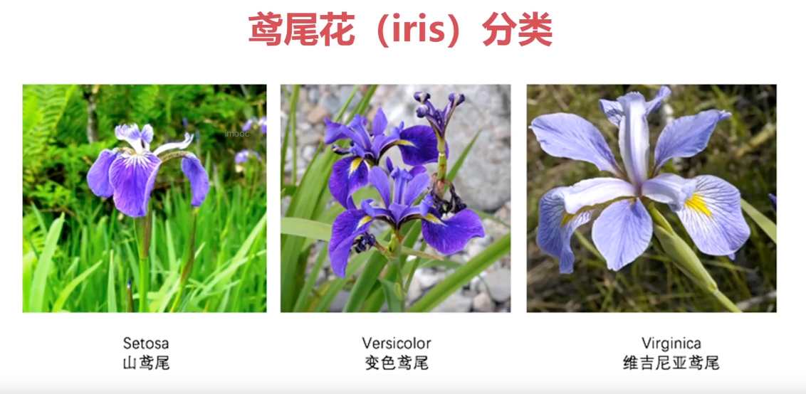
export const IRIS_CLASSES =
['山鸢尾', '变色鸢尾', '维吉尼亚鸢尾'];
export const IRIS_NUM_CLASSES = IRIS_CLASSES.length;

// Iris flowers data. Source:
// https://archive.ics.uci.edu/ml/machine-learning-databases/iris/iris.data
const IRIS_DATA = [
[5.1, 3.5, 1.4, 0.2, 0], [4.9, 3.0, 1.4, 0.2, 0], [4.7, 3.2, 1.3, 0.2, 0],
[4.6, 3.1, 1.5, 0.2, 0], [5.0, 3.6, 1.4, 0.2, 0], [5.4, 3.9, 1.7, 0.4, 0],
[4.6, 3.4, 1.4, 0.3, 0], [5.0, 3.4, 1.5, 0.2, 0], [4.4, 2.9, 1.4, 0.2, 0],
[4.9, 3.1, 1.5, 0.1, 0], [5.4, 3.7, 1.5, 0.2, 0], [4.8, 3.4, 1.6, 0.2, 0],
[4.8, 3.0, 1.4, 0.1, 0], [4.3, 3.0, 1.1, 0.1, 0], [5.8, 4.0, 1.2, 0.2, 0],
[5.7, 4.4, 1.5, 0.4, 0], [5.4, 3.9, 1.3, 0.4, 0], [5.1, 3.5, 1.4, 0.3, 0],
[5.7, 3.8, 1.7, 0.3, 0], [5.1, 3.8, 1.5, 0.3, 0], [5.4, 3.4, 1.7, 0.2, 0],
[5.1, 3.7, 1.5, 0.4, 0], [4.6, 3.6, 1.0, 0.2, 0], [5.1, 3.3, 1.7, 0.5, 0],
[4.8, 3.4, 1.9, 0.2, 0], [5.0, 3.0, 1.6, 0.2, 0], [5.0, 3.4, 1.6, 0.4, 0],
[5.2, 3.5, 1.5, 0.2, 0], [5.2, 3.4, 1.4, 0.2, 0], [4.7, 3.2, 1.6, 0.2, 0],
[4.8, 3.1, 1.6, 0.2, 0], [5.4, 3.4, 1.5, 0.4, 0], [5.2, 4.1, 1.5, 0.1, 0],
[5.5, 4.2, 1.4, 0.2, 0], [4.9, 3.1, 1.5, 0.1, 0], [5.0, 3.2, 1.2, 0.2, 0],
[5.5, 3.5, 1.3, 0.2, 0], [4.9, 3.1, 1.5, 0.1, 0], [4.4, 3.0, 1.3, 0.2, 0],
[5.1, 3.4, 1.5, 0.2, 0], [5.0, 3.5, 1.3, 0.3, 0], [4.5, 2.3, 1.3, 0.3, 0],
[4.4, 3.2, 1.3, 0.2, 0], [5.0, 3.5, 1.6, 0.6, 0], [5.1, 3.8, 1.9, 0.4, 0],
[4.8, 3.0, 1.4, 0.3, 0], [5.1, 3.8, 1.6, 0.2, 0], [4.6, 3.2, 1.4, 0.2, 0],
[5.3, 3.7, 1.5, 0.2, 0], [5.0, 3.3, 1.4, 0.2, 0], [7.0, 3.2, 4.7, 1.4, 1],
[6.4, 3.2, 4.5, 1.5, 1], [6.9, 3.1, 4.9, 1.5, 1], [5.5, 2.3, 4.0, 1.3, 1],
[6.5, 2.8, 4.6, 1.5, 1], [5.7, 2.8, 4.5, 1.3, 1], [6.3, 3.3, 4.7, 1.6, 1],
[4.9, 2.4, 3.3, 1.0, 1], [6.6, 2.9, 4.6, 1.3, 1], [5.2, 2.7, 3.9, 1.4, 1],
[5.0, 2.0, 3.5, 1.0, 1], [5.9, 3.0, 4.2, 1.5, 1], [6.0, 2.2, 4.0, 1.0, 1],
[6.1, 2.9, 4.7, 1.4, 1], [5.6, 2.9, 3.6, 1.3, 1], [6.7, 3.1, 4.4, 1.4, 1],
[5.6, 3.0, 4.5, 1.5, 1], [5.8, 2.7, 4.1, 1.0, 1], [6.2, 2.2, 4.5, 1.5, 1],
[5.6, 2.5, 3.9, 1.1, 1], [5.9, 3.2, 4.8, 1.8, 1], [6.1, 2.8, 4.0, 1.3, 1],
[6.3, 2.5, 4.9, 1.5, 1], [6.1, 2.8, 4.7, 1.2, 1], [6.4, 2.9, 4.3, 1.3, 1],
[6.6, 3.0, 4.4, 1.4, 1], [6.8, 2.8, 4.8, 1.4, 1], [6.7, 3.0, 5.0, 1.7, 1],
[6.0, 2.9, 4.5, 1.5, 1], [5.7, 2.6, 3.5, 1.0, 1], [5.5, 2.4, 3.8, 1.1, 1],
[5.5, 2.4, 3.7, 1.0, 1], [5.8, 2.7, 3.9, 1.2, 1], [6.0, 2.7, 5.1, 1.6, 1],
[5.4, 3.0, 4.5, 1.5, 1], [6.0, 3.4, 4.5, 1.6, 1], [6.7, 3.1, 4.7, 1.5, 1],
[6.3, 2.3, 4.4, 1.3, 1], [5.6, 3.0, 4.1, 1.3, 1], [5.5, 2.5, 4.0, 1.3, 1],
[5.5, 2.6, 4.4, 1.2, 1], [6.1, 3.0, 4.6, 1.4, 1], [5.8, 2.6, 4.0, 1.2, 1],
[5.0, 2.3, 3.3, 1.0, 1], [5.6, 2.7, 4.2, 1.3, 1], [5.7, 3.0, 4.2, 1.2, 1],
[5.7, 2.9, 4.2, 1.3, 1], [6.2, 2.9, 4.3, 1.3, 1], [5.1, 2.5, 3.0, 1.1, 1],
[5.7, 2.8, 4.1, 1.3, 1], [6.3, 3.3, 6.0, 2.5, 2], [5.8, 2.7, 5.1, 1.9, 2],
[7.1, 3.0, 5.9, 2.1, 2], [6.3, 2.9, 5.6, 1.8, 2], [6.5, 3.0, 5.8, 2.2, 2],
[7.6, 3.0, 6.6, 2.1, 2], [4.9, 2.5, 4.5, 1.7, 2], [7.3, 2.9, 6.3, 1.8, 2],
[6.7, 2.5, 5.8, 1.8, 2], [7.2, 3.6, 6.1, 2.5, 2], [6.5, 3.2, 5.1, 2.0, 2],
[6.4, 2.7, 5.3, 1.9, 2], [6.8, 3.0, 5.5, 2.1, 2], [5.7, 2.5, 5.0, 2.0, 2],
[5.8, 2.8, 5.1, 2.4, 2], [6.4, 3.2, 5.3, 2.3, 2], [6.5, 3.0, 5.5, 1.8, 2],
[7.7, 3.8, 6.7, 2.2, 2], [7.7, 2.6, 6.9, 2.3, 2], [6.0, 2.2, 5.0, 1.5, 2],
[6.9, 3.2, 5.7, 2.3, 2], [5.6, 2.8, 4.9, 2.0, 2], [7.7, 2.8, 6.7, 2.0, 2],
[6.3, 2.7, 4.9, 1.8, 2], [6.7, 3.3, 5.7, 2.1, 2], [7.2, 3.2, 6.0, 1.8, 2],
[6.2, 2.8, 4.8, 1.8, 2], [6.1, 3.0, 4.9, 1.8, 2], [6.4, 2.8, 5.6, 2.1, 2],
[7.2, 3.0, 5.8, 1.6, 2], [7.4, 2.8, 6.1, 1.9, 2], [7.9, 3.8, 6.4, 2.0, 2],
[6.4, 2.8, 5.6, 2.2, 2], [6.3, 2.8, 5.1, 1.5, 2], [6.1, 2.6, 5.6, 1.4, 2],
[7.7, 3.0, 6.1, 2.3, 2], [6.3, 3.4, 5.6, 2.4, 2], [6.4, 3.1, 5.5, 1.8, 2],
[6.0, 3.0, 4.8, 1.8, 2], [6.9, 3.1, 5.4, 2.1, 2], [6.7, 3.1, 5.6, 2.4, 2],
[6.9, 3.1, 5.1, 2.3, 2], [5.8, 2.7, 5.1, 1.9, 2], [6.8, 3.2, 5.9, 2.3, 2],
[6.7, 3.3, 5.7, 2.5, 2], [6.7, 3.0, 5.2, 2.3, 2], [6.3, 2.5, 5.0, 1.9, 2],
[6.5, 3.0, 5.2, 2.0, 2], [6.2, 3.4, 5.4, 2.3, 2], [5.9, 3.0, 5.1, 1.8, 2],
];

/**
* Convert Iris data arrays to `tf.Tensor`s.
*
* @param data The Iris input feature data, an `Array` of `Array`s, each element
* of which is assumed to be a length-4 `Array` (for petal length, petal
* width, sepal length, sepal width).
* @param targets An `Array` of numbers, with values from the set {0, 1, 2}:
* representing the true category of the Iris flower. Assumed to have the same
* array length as `data`.
* @param testSplit Fraction of the data at the end to split as test data: a
* number between 0 and 1.
* @return A length-4 `Array`, with
* - training data as `tf.Tensor` of shape [numTrainExapmles, 4].
* - training one-hot labels as a `tf.Tensor` of shape [numTrainExamples, 3]
* - test data as `tf.Tensor` of shape [numTestExamples, 4].
* - test one-hot labels as a `tf.Tensor` of shape [numTestExamples, 3]
*/
function convertToTensors(data, targets, testSplit) {
const numExamples = data.length;
if (numExamples !== targets.length) {
throw new Error('data and split have different numbers of examples');
}

// Randomly shuffle `data` and `targets`.
const indices = [];
for (let i = 0; i < numExamples; ++i) {
indices.push(i);
}
tf.util.shuffle(indices);

const shuffledData = [];
const shuffledTargets = [];
for (let i = 0; i < numExamples; ++i) {
shuffledData.push(data[indices[i]]);
shuffledTargets.push(targets[indices[i]]);
}

// Split the data into a training set and a tet set, based on `testSplit`.
const numTestExamples = Math.round(numExamples * testSplit);
const numTrainExamples = numExamples - numTestExamples;

const xDims = shuffledData[0].length;

// Create a 2D `tf.Tensor` to hold the feature data.
const xs = tf.tensor2d(shuffledData, [numExamples, xDims]);

// Create a 1D `tf.Tensor` to hold the labels, and convert the number label
// from the set {0, 1, 2} into one-hot encoding (.e.g., 0 --> [1, 0, 0]).
const ys = tf.oneHot(tf.tensor1d(shuffledTargets).toInt(), IRIS_NUM_CLASSES);

// Split the data into training and test sets, using `slice`.
const xTrain = xs.slice([0, 0], [numTrainExamples, xDims]);
const xTest = xs.slice([numTrainExamples, 0], [numTestExamples, xDims]);
const yTrain = ys.slice([0, 0], [numTrainExamples, IRIS_NUM_CLASSES]);
const yTest = ys.slice([0, 0], [numTestExamples, IRIS_NUM_CLASSES]);
return [xTrain, yTrain, xTest, yTest];
}

/**
* Obtains Iris data, split into training and test sets.
*
* @param testSplit Fraction of the data at the end to split as test data: a
* number between 0 and 1.
*
* @param return A length-4 `Array`, with
* - training data as an `Array` of length-4 `Array` of numbers.
* - training labels as an `Array` of numbers, with the same length as the
* return training data above. Each element of the `Array` is from the set
* {0, 1, 2}.
* - test data as an `Array` of length-4 `Array` of numbers.
* - test labels as an `Array` of numbers, with the same length as the
* return test data above. Each element of the `Array` is from the set
* {0, 1, 2}.
*/
export function getIrisData(testSplit) {
return tf.tidy(() => {
const dataByClass = [];
const targetsByClass = [];
for (let i = 0; i < IRIS_CLASSES.length; ++i) {
dataByClass.push([]);
targetsByClass.push([]);
}
for (const example of IRIS_DATA) {
const target = example[example.length - 1];
const data = example.slice(0, example.length - 1);
dataByClass[target].push(data);
targetsByClass[target].push(target);
}

const xTrains = [];
const yTrains = [];
const xTests = [];
const yTests = [];
for (let i = 0; i < IRIS_CLASSES.length; ++i) {
const [xTrain, yTrain, xTest, yTest] =
convertToTensors(dataByClass[i], targetsByClass[i], testSplit);
xTrains.push(xTrain);
yTrains.push(yTrain);
xTests.push(xTest);
yTests.push(yTest);
}

const concatAxis = 0;
return [
tf.concat(xTrains, concatAxis), tf.concat(yTrains, concatAxis),
tf.concat(xTests, concatAxis), tf.concat(yTests, concatAxis)
];
});
}

script.js

1
2
3
4
5
6
7
8
9
10
11
12
13
14
15
16
17
18
19
20
21
22
23
24
25
26
27
28
29
30
31
32
33
34
35
36
37
38
39
40
41
42
43
44
45
46
import * as tf from '@tensorflow/tfjs';
import * as tfvis from '@tensorflow/tfjs-vis';
import { getIrisData, IRIS_CLASSES } from './data';

window.onload = async () => {
const [xTrain, yTrain, xTest, yTest] = getIrisData(0.15); // 15% 的数据用作验证集

const model = tf.sequential();
model.add(tf.layers.dense({
units: 10,
inputShape: [xTrain.shape[1]],
activation: 'sigmoid'
}));
model.add(tf.layers.dense({
units: 3,
activation: 'softmax'
}));

model.compile({
loss: 'categoricalCrossentropy',
optimizer: tf.train.adam(0.1),
metrics: ['accuracy']
});

await model.fit(xTrain, yTrain, {
epochs: 100,
validationData: [xTest, yTest], // 验证集
callbacks: tfvis.show.fitCallbacks(
{ name: '训练效果' },
['loss', 'val_loss', 'acc', 'val_acc'],
{ callbacks: ['onEpochEnd'] }
)
});

window.predict = (form) => {
const input = tf.tensor([[
form.a.value * 1,
form.b.value * 1,
form.c.value * 1,
form.d.value * 1,
]]);
const pred = model.predict(input);
alert(`预测结果:${IRIS_CLASSES[pred.argMax(1).dataSync(0)]}`);
};
};

index.html

1
2
3
4
5
6
7
8
9
<script src="script.js"></script>
<form action="" onsubmit="predict(this); return false;">
花萼长度:<input type="text" name="a"><br>
花萼宽度:<input type="text" name="b"><br>
花瓣长度:<input type="text" name="c"><br>
花瓣宽度:<input type="text" name="d"><br>
<button type="submit">预测</button>
</form>


欠拟合

数据很复杂,模型太简单了,拟合不了这个数据

上图中黑色的线代表的数据,蓝色线是我们的模型,显然蓝色的模型不能拟合黑色的数据,这种情况就叫欠拟合

过拟合

模型太过复杂,新数据验证的效果不好

上图中红色的点和蓝色的点代表两类数据,黑色的线代表正常的模型,绿色的线就是过拟合的模型,模型的形态比较混乱

经典的过拟合曲线 (红色代表验证集的损失,蓝色的线代表训练集的损失)

训练数据简单,模型太过复杂

应对过拟合的方法:

  1. 早停法
  2. 权重衰减法 kernelRegularizer: tf.regularizers.l2({ l2: 1 })
  3. 丢弃法 model.add(tf.layers.dropout({ rate: 0.9 })); 是在神经网络模型中添加一个 dropout 层,用于防止过拟合。
    等。。。

欠拟合代码

script.js

1
2
3
4
5
6
7
8
9
10
11
12
13
14
15
16
17
18
19
20
21
22
23
24
25
26
27
28
29
30
31
32
33
34
35
36
37
38
39
40
41
42
43
44
45

import * as tf from '@tensorflow/tfjs';
import * as tfvis from '@tensorflow/tfjs-vis';
import { getData } from '../xor/data';

window.onload = async () => {
const data = getData(200);

tfvis.render.scatterplot(
{ name: '训练数据' },
{
values: [
data.filter(p => p.label === 1),
data.filter(p => p.label === 0),
]
}
);

const model = tf.sequential();
model.add(tf.layers.dense({
units: 1,
inputShape: [2],
activation: "sigmoid",
// kernelRegularizer: tf.regularizers.l2({ l2: 1 })
}));

model.compile({
loss: tf.losses.logLoss,
optimizer: tf.train.adam(0.1)
});

const inputs = tf.tensor(data.map(p => [p.x, p.y]));
const labels = tf.tensor(data.map(p => p.label));

await model.fit(inputs, labels, {
validationSplit: 0.2,
epochs: 200,
callbacks: tfvis.show.fitCallbacks(
{ name: '训练效果' },
['loss', 'val_loss'],
{ callbacks: ['onEpochEnd'] }
)
});
};

过拟合代码

data.js 带有噪音的二分类数据

1
2
3
4
5
6
7
8
9
10
11
12
13
14
15
16
17
18
19
20
21
22
23
24
25
26
27
28
29
30
31
32
33
34
35
export function getData(numSamples, variance) {
let points = [];

function genGauss(cx, cy, label) {
for (let i = 0; i < numSamples / 2; i++) {
let x = normalRandom(cx, variance);
let y = normalRandom(cy, variance);
points.push({ x, y, label });
}
}

genGauss(2, 2, 1);
genGauss(-2, -2, 0);
return points;
}

/**
* Samples from a normal distribution. Uses the seedrandom library as the
* random generator.
*
* @param mean The mean. Default is 0.
* @param variance The variance. Default is 1.
*/
function normalRandom(mean = 0, variance = 1) {
let v1, v2, s;
do {
v1 = 2 * Math.random() - 1;
v2 = 2 * Math.random() - 1;
s = v1 * v1 + v2 * v2;
} while (s > 1);

let result = Math.sqrt(-2 * Math.log(s) / s) * v1;
return mean + Math.sqrt(variance) * result;
}

script.js

1
2
3
4
5
6
7
8
9
10
11
12
13
14
15
16
17
18
19
20
21
22
23
24
25
26
27
28
29
30
31
32
33
34
35
36
37
38
39
40
41
42
43
44
45
46
47
48
49

import * as tf from '@tensorflow/tfjs';
import * as tfvis from '@tensorflow/tfjs-vis';
import { getData } from './data';

window.onload = async () => {
const data = getData(200, 2);

tfvis.render.scatterplot(
{ name: '训练数据' },
{
values: [
data.filter(p => p.label === 1),
data.filter(p => p.label === 0),
]
}
);

const model = tf.sequential();
model.add(tf.layers.dense({
units: 10,
inputShape: [2],
activation: "tanh",
// kernelRegularizer: tf.regularizers.l2({ l2: 1 })
}));
model.add(tf.layers.dropout({ rate: 0.9 }));
model.add(tf.layers.dense({
units: 1,
activation: 'sigmoid'
}));
model.compile({
loss: tf.losses.logLoss,
optimizer: tf.train.adam(0.1)
});

const inputs = tf.tensor(data.map(p => [p.x, p.y]));
const labels = tf.tensor(data.map(p => p.label));

await model.fit(inputs, labels, {
validationSplit: 0.2,
epochs: 200,
callbacks: tfvis.show.fitCallbacks(
{ name: '训练效果' },
['loss', 'val_loss'],
{ callbacks: ['onEpochEnd'] }
)
});
};

index.html

1
2
3

<script src="script.js"></script>

设置权重衰减:kernelRegularizer: tf.regularizers.l2({ l2: 1 }) 结果如下图

参考:

https://playground.tensorflow.org/#activation=tanh&batchSize=10&dataset=circle&regDataset=reg-plane&learningRate=0.03&regularizationRate=0&noise=0&networkShape=4,2&seed=0.94941&showTestData=false&discretize=false&percTrainData=50&x=true&y=true&xTimesY=false&xSquared=false&ySquared=false&cosX=false&sinX=false&cosY=false&sinY=false&collectStats=false&problem=classification&initZero=false&hideText=false

https://js.tensorflow.org/api/latest/?hl=zh-cn&_gl=1*nv702p*_ga*MjExOTY1MjIyNi4xNzQ1ODI3MTc0*_ga_W0YLR4190T*MTc0NTgzMTA0MC4yLjEuMTc0NTgzMjU4OC4wLjAuMA..#dot

google机器学习课程 course
https://developers.google.com/machine-learning/crash-course/linear-regression?hl=zh-cn

https://www.bilibili.com/video/BV1p2BWYVEik?spm_id_from=333.788.player.switch&vd_source=ffda878df0ed45bee1ade91d8f451048&p=10

kimi问答
https://kimi.moonshot.cn/chat/d0dcjumf2kqelc31foc0

https://ml-cheatsheet.readthedocs.io/en/latest/loss_functions.html?highlight=cross#cross-entropy